Manual of the Freiburg Vision Test  ‘FrACT₁₀’  Vs. 2024-03-31

This manual describes ‘FrACT₁₀’, which appeared in a usable version in April 2020. It will eventually supersede the classic FrACT, now at version 3.10.5. FrACT₁₀ is a rewrite that runs on all platforms in all current browsers, because it is based on Cappuccino, in turn based on JavaScript all the way down. It inherited all algorithms from the classic FrACT (Bach 1996, 1997, 2007). At the same time, some design decisions were revisited: The export format is more systematic, optotype contrast is in Weber units, etc.; also operation on touch devices is now possible (if large enough, e.g. tablets). FrACT₁₀ is currently on-line only.

This manual assumes that the user has a working knowledge of the principles and practice of the assessment of human visual acuity. FrACT₁₀ is freely accessible here.

Two things need to be calibrated in Settings▸︎General

1. The observation distance. Measure from screen to eye; enter value at the Settings screen in centimeters. And make sure this distance is being kept throughout the test.
2. The length of the blue ruler line on the Settings screen (no need for a ruler with the plastic-card approach). This allows the program to calculate the screen resolution (pixels per mm). Don’t change the zoom level of your browser or the operating system after calibration, obviously.

The above two settings together allow the program to calculate the correct visual angle of the optotypes. Usually, the pixel size limits the maximal acuity, and can be a severe limit for near vision assessment. Thus, on the bottom right “→max possible decimal acuity” resp. “→min possible LogMAR” shows what can be reached, assuming minimal gap/stroke size is 1 pixel. Actually, minimal gap/stroke size can be 0.5 through antialiasing, thus better acuities may result.

FrACT unfortunately has too often been used without calibration. Thus this intentionally annoying message appears on the beginning of every run, unless you have changed both the observer distance entry and the length of the blue calibration ruler (see preceding paragraph). Both are defaulted to numbers that are unlikely to occur in practice (149 mm and 399 cm). So: calibrate! It’s easy. For more see section Calibration.

There are many possibilities to measure the ‘minimum visibile’, a common and sensible approach is to present an “optotype”, be it a Sloan letter, a tumbling E or a Landolt ring (=Landolt C).

The basic procedure starts with a very large (= easy to recognize) optotype, and having the participant or patient indicate recognition (e.g., name the letter, name the orientation of the gap in the Landolt C). Depending on the correctness of the response, next an easier or more difficult to recognize optotype is presented, ultimately aiming to determine the spatial resolution limit or threshold. Since there is a gradual loss of likelihood to respond correctly with decreasing size, the threshold must be consider a probability. The best choice is to set the threshold recognition rate in the middle between 100% and the guessing rate (12.5% in the case of 8 choices), 56.25% for this example. This means that at the “acuity value” nearly half the optotypes are not recognized correctly. This may initially appear counter-intuitive.

An additional procedural detail is the “forced choice” principle: The participant needs to respond even if they cannot make out the optotype at all. They have to give their best guess, which may be random. This is a way to reduce the influence of the “response criterion”, that is whether the participant is timid (only responding when absolutely certain) or dashing (making wild guesses). Thus incorrect responses will enter into the procedure, which also may appear counter-intuitive.

To control the sequence of optotype presented and to arrive at a threshold estimate, FrACT₁₀ currently employs the “Best PEST” procedure. This means that the program determines the most likely estimate of the threshold, given the optotype grades and responses so far, and then presents the optotype exactly at the current threshold estimate, thus maximizing information gain.

In the first 4 trials, the Best Pest is overridden (following EN ISO) by the values 0.1, 0.2, 0.4, 0.8, as long as the responses are correct. This also avoids extremely difficult optotypes after a correct initial response.

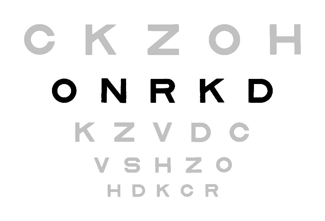
Acuity assessed with Sloan Letters

Based on Louise Sloan (1959), these 10 letters are used: CDHKNORSVZ; these are also used in the ETDRS charts. In FrACT₁₀ the Sloan Letters are drawn by vector graphics that I based on the detailed description (Committee on Vision 1980), not on the slightly incorrect “Sloan font”. To respond, the participant (or operator) types the appropriate letter on the keyboard (or touches the corresponding button). Any non-Sloan letter is considered an incorrect response.

Acuity with the Landolt ring = Landolt C

The Landolt C is the gold-standard optotype (International Organization for Standardization 2017). It can be presented in one of 8 different orientations. [Or 4, if so chosen in Settings▸General]. An advantage of Landolt Cs: no literacy is required. With 8 orientations, the guessing rate is 12.5%, close to the 10% with Sloan Letters. When only 4 orientations are employed, more trials are necessary.

Acuity with the Tumbling E

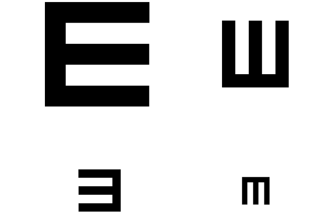
The E shape in the tumbling E has the same basic dimensions as the Landolt C, but is only presented in one out of 4 possible orientations. The Tumbling E is a classic optotype. A slight disadvantage compared to the Landolt C is a wee more luminance imbalance close to the threshold – this is relevant when considering recognition vs. discrimination acuity.

Acuity with TAO (The Auckland Optotypes)

These optotypes are useful for infant assessment and are available in 10 different shapes. See this this paper: Hamm et al. (2018) for a careful evaluation of TAO (The Auckland Optotypes) results. Currently TAO can only run at 100% contrast, and the response keys are less intuitive; thus there is a legend at the bottom of the test screen.

Vernier acuity

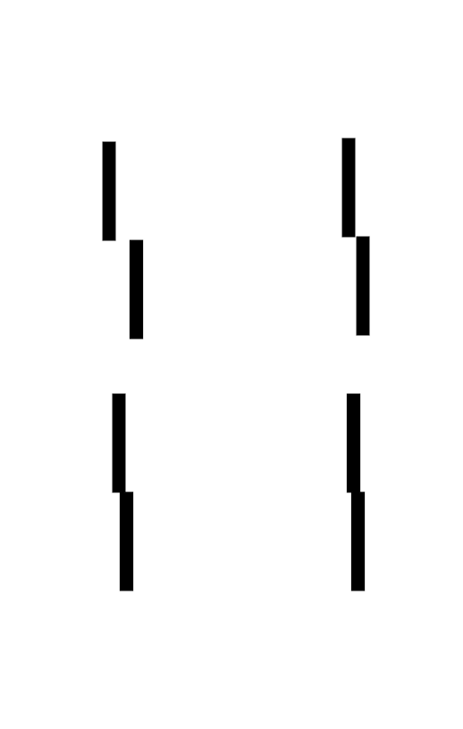
Vernier acuity is nearly 10× better than optotype acuity. In FrACT₁₀, Vernier acuity is based on line-segment alignment, 2-line or 3-line arrangements can be chosen. Since only 2 choices are possible, many trials are necessary; the default setting is the lowest limit, more is better. Enter the displacement of the upper line relative to the lower line through the cursor keys or the digits 4 / 6. Since Vernier acuity is so high, the considerations in “Note on display resolutions” (below) are particularly pertinent – you may need 10× higher distance to your display unit.

Line of optotypes

In contrast to the other test modes, “Line of optotypes” or “Line-by-line” does not offer automatic testing. Instead, this mode displays a line of five optotypes, Sloan letters or Landolt Cs. Initially the acuity grade is 0.3 LogMAR. Using the ↑↓ cursor keys it can be changed in 0.1 LogMAR steps throughout the range possible given VDU size and distance. The ⇄ cursor keys reshuffle the optotypes into a new random selection. The inter-optotype distance can be set to either DIN-EN-ISO or ETRDS like (details below in Settings▸Acuity).

This module (added on request) allows to operate FrACT₁₀ akin to a chart. It’s even easier because only one line is presented at a time. Furthermore, this mode provides a useful target when optimising refraction. With the setting Chart mode its’s more similar to a conventional chart (and implies vertical crowding).

Nomenclature

There exist (too many) traditions to format visual acuity: LogMAR, decimal, Snellen fraction; FrACT₁₀ caters for these three. Whichever of these measures you prefer, they can be easily converted into each other when distance is known. Details and conversion tables are given here.

Limitations in accessible acuity

There are technical limits on the highest and lowest acuity, which depend on the display resolution in pixels per inch, VDU size, and on the distance. For distances of ≥ 3 m the normal monitor resolution (≈ 72 dots per inch) is fine. Lower distances only work with devices that have very high spatial resolution (e.g. OLEDs, readily available now) or in low acuity situations, see “Note on display resolutions” (below). If you want to assess low vision (LogMAR 1.0, decimal 0.1 = 20/200 and worse), a distance to the display of 0.5–1.0 m is sufficient (possibly necessary, in addition to a large screen).

The term “contrast sensitivity” (CS) lets many people reflexively think of sine-wave gratings. Gratings allow to assess CS for a specific spacial frequency. While this is fine, there is no clinical condition which leads to specific loss of intermediate spatial frequencies, rendering moot the specific measurement at various spatial frequencies.

Primarily, like the Pelli-Robson or the Mars charts, FrACT₁₀ assesses contrast using standard optotypes. These are composed of a mixture of low to medium spatial frequencies (as can be determined via a Fourier analysis). At the high spatial frequency end, CS and visual acuity tap the same physiological bottleneck, so acuity alone is sufficient there. This saves precious measurement time.
Thus, FrACT₁₀ assesses contrast sensitivity by displaying medium large optotypes at fixed size. Depending on the responses o the testee, the contrast is reduced following a Best PEST procedure like for visual acuity to assess the threshold using a Bayes-like approach. Since dithering allows very low contrasts, the maximal result is clamped at 2.0 logCSweber, beyond the physiological range.

There is also the option to use gratings. They are presented in four possible orientations (or, optionally 2). Correct responses to the orientations reduce the contrast of the next presentation following the algorithm mentioned above. To correctly assess the human contrast threshold within the limitations of 8-bit greyscale dept, error diffusion is employed. A recent addition to Gratings allows to also assess the upper spatial frequency limit (“grating acuity”). This is intricate and not discussed here.

Contrast formats

First, Contrast Sensitivity is the reciprocal value of the threshold contrast. Thus, if the just visible contrast (the threshold contrast) is very small, then the contrast sensitivity is high. Unfortunately, there are 4 (four!) different definitions of contrast in use. Of these, FrACT reports the Weber contrast for all optotypes (in logCS), and Michelson contrast (in percent) for gratings.

Which size for the contrast optotype?

There is a wild variety in the literature…

I conducted the above overview 2024-02 (with kind advice from John Robson) and consequently increased the default size from 50 to 170 arcmin (≙2.85°). Now the default complies with the most common Pelli-Robson chart usage and is within a factor of ≈2 of the Mars chart.

Limitations in contrast testing

1. Assessment of the contrast threshold requires good gamma correction (display linearization). The best approach is to use a dedicated screen calibrator (e.g. Spyder by DataColor) to set system gamma to 1.0 and then set FrACT₁₀’s gamma to 1.0 as well (on the screen Settings▸Contrast).
2. Display limitations. Most current visual display units (LCDs etc.) have a luminance resolution of 8 bit per primary colour. Thus there are only 256 levels, or about half as many after gamma correction. This is insufficient to display a real threshold stimulus for good vision. There are 3 ways to deal with it:
   1. Use dithering. Since 2023-04-01 it’s by default on in FrACT₁₀, this allows contrasts higher then 2.0 logCSweber, beyond the physiological range.
   2. Ignore it. The achievable value for the contrast sensitivity of over 1.6 logCSweber, which is “good enough” for most purposes. Participants with this value clearly have good contrast vision.
   3. Use “error diffusion” {default: on} with gratings. With that technique, gratings can assess the human threshold.
   4. Use colour-bit stealing. This was implemented in FrACT3, but deactivated because it can’t work in colour anopia. Available in FrACT₁₀, but not good enough yet (has color artifacts). Not necessary, we have dithering.
      
      Summarising: With dithering, FrACT₁₀ can assess contrast sensitivity across the full physiological range.
3. Distance is not so critical as for acuity, since the optotype’s size typically is markedly above the spatial resolution limit. 1 m or more is fine.

Numerous options have been added to FrACT over the years, often on user request. The following list follows the sequence in FrACT₁₀’s “Settings” dialog, which is segregated into the tabs «General | Acuity | Contrast | Gamma».
If any fields are empty, reload. ← 2021-07-04 should not occur any more, but the rule is still fine :)

# of choices and # of trials

The # of choices for Landolt Cs and gratings

Different optotypes have a different number of choices (or alternatives, or orientations): Sloan Letters have always 10 choices, Tumbling E always 4, hyperacuity (Vernier) always 2. For Landolt Cs it can be selected between 4 and 8 {default: 8}, for gratings between 2 and 3 {default: 4}. The threshold algorithm always uses the appropriate guessing rate of 10%, 12.5%, 25% or 50% respectively. If 4 choices is selected, an additional option Oblique only appears; this is useful only with Landolt Cs.
These values apply for both acuity and contrast assessment.

The # of trials {for 2 / 4 / 8 choices}

The number of trials can be set to any reasonable number. A multiple of 6 (e.g., 18 or 24) is preferred so that the last trial is a “bonus trial” (see below), leaving the participant with a success experience for the last trial. The number of trials is separate for the 2 vs. 4 vs. 8 direction conditions, because more choices require fewer trials for comparable accuracy. For the hyperacuity test, there are only 2 possible choices. Tumbling E will use the 4 choices selection, the trial number of the Sloan letters will be based on the 8 choices selection (because the guessing rates of 12.5% and 10% do not differ much) {defaults: 32 / 24 / 18}.

Timeouts

There are two timeouts, one controls the time the optotype remains visible, the other limits reaction time.

• Display time can be limited to a certain number of seconds from 0.1 to 999; when exceeded, the optotype disappears.
• Response time can be limited to a certain number of seconds from 1 to 999, e.g. 10 s; when exceeded, an incorrect response is assumed and a new trial is started. Such time limitation was required for a European traffic expertise (not any more). Ten seconds can already be challenging for elderly participants {defaults: 30 s / 30 s}

Show operation info at start of each run

If enabled, a brief explanation of the response keys appears at he beginning of each run. Switch off, of course, as soon as you’re experienced {default: «on»}.

Enable touch controls

To enable FrACT₁₀ on tablets without a keyboard, touch buttons can be shown {default: «on»}.

Show info (top left) each trial

When on, shows current trial number, total number of trials, and the current threshold (acuity: in decimal) in tiny letters at top left {default: «on»}.

Which test on ‘5’

For extended measurements, it can be useful to control everything through the remote keypad (see the note on response keys below). This setting selects which test is started by pressing the central ‘5’ key. Options are: «None | Sloan Letters | Landolt C | Tumbling E | TAO | Hyperacuity | …» {default: Sloan Letters}.

Results to clipboard

See below for a detailed discussion of results export. Briefly here: After each run, one can –without quitting FrACT₁₀– switch to a concurrently running spreadsheet and paste-in the run details (see below for a full format specification). When the “full history” option is chosen [does not work yet], for each trial the presented orientation, responded orientation, and reaction time are provided as well. [The clipboard is the place in the computer were any copy or cut operation places its result, ready to be pasted elsewhere.] For correct transfer of data, you must set the appropriate character (for your country) for the decimal separator beforehand (“automatic” may be enough, see next items)!

When this setting is on, one is reminded after each run to place the result on the clipboard and then one can use the task switcher to select a spreadsheet already running in the background. When this setting is off, it is still possible to use the button Export→Clipboard that will appear on the right after each run. That button can be ignored, of course.

Why are there both options, the “Export results to clipboard” not set to “None”, and the separate export button? While the latter would, in principle, suffice, it is very easy to forget, and loosing the result. On the other hand, for a try-out, it’s handy to have the button without a dialog getting into the way,

Options are: «None / Final results only / Full trial history», default: «None»}.

“silently” checkbox

If enabled, and “Export…” is not None, the results are copied to the clipboard without asking first. On one hand this is faster (one click less), on the other it’s easier to forget to transfer the obtained results to a spreadsheet {default: «off»}.
Depending on your browser’s security settings, this might not work.

Decimal separator

Different countries use different number formatting; furthermore different post-processing programs can require different formatting. The setting for the decimal separator, a point or a comma, applies both to the clipboard exports and to the large result display after a finished run (not to the local storage export). Be sure to select the right value, otherwise Excel might convert your results to dates! {Default: ‘automatic’}

Use mobile orientation

When running on a tablet / smartphone (latter not endorsed), this will cause a reload of FrACT₁₀ when rotating the device by 90°. That allows the window to fit fully on the screen.

Display transformation

To increase observation distance, mirror arrangements (high-quality front surface, of course) or afocal telescopes can be used. Since these can flip the orientation, corrective transformations can be applied. Options are: «normal | mirror horizontally | mirror vertically | rotate by 180°» {default: normal}.

Feedback

It is usually advised not to give feedback on correctness, likely sensible for human-human interaction; however this was never tested until Bach & Schäfer K (2016). There we found that for typical clinical trials (up to 6 runs at 24 trials each) feedback does not affect the results nor reproducibility, but markedly enhances participant comfort. So in FrACT₁₀ you have the choice: The participant’s response can be acoustically announced through a short tone, options are: «None | Always | On correct | With info». “With info”: two different sounds on correct/incorrect {default: «With info»}.

The option “Auditory feedback at end” allows to emit a “success sound” when the last trial has been responded to. Options are: «off / on» {default: «on»}.

The slider allows to adjust the sound volume from 1 to 100% {default: 20%}. Test with the button designated with the loudspeaker.

Finally, “Reward pictures at end” allows to present a “nice” picture at the end of a non-aborted run {default: «off»}. Particularly useful for children testing, but I like it too. During presentation of the picture the underlying buttons can still be clicked. When this option is on, the duration of the picture can be adjusted, defaulting to 5 seconds.

In summary, various feedback actions default to «on», but can all be shut off if deemed to distracting or annoying.

Optotype eccentricity

The optotypes can be displaced relative to the center of the screen {default: (0°, 0°)}. This allows for systematic variation of eccentricity. The touch controls (if visible) stay in place, so on small screens overlap can occur. An optional center fixation mark helps to fixate {default: «on»}. It only appears if it does not overlap with the optotype.

Calibrate with plastic card et.

See section Size Calibration.

Optotypes / background color

Depending on the radio button state at left, the optotype and background colors are either grey levels (b/w) and defined via contrast, or any value as selected in the color wells.

b/w

Monitor hood reduces stray light.

For acuity testing, the contrast value of the optotype must be near 100% for the standard (ISO) definition of visual acuity; its value can be set from 1%–100% for specific questions. For precise contrast presentation, stray light must be avoided and VDU-gamma must be set correctly as appropriate for your sytem (see Settings▸Gamma). Contrast is entered in Weber (!) format, see explanation and conversion formulae below. Negative values: inverted optotype (light optotype on dark background). Please note: since it’s in Weber contrast units, a white-on-black optotype needs -∞% contrast (approximated, e.g., by -10000%; see max± buttons). {default: 100%}.

Color

Here custom colors can be selected via the color wells. In its sliders subpanes, you can enter quantitative hex values. There are two glitches here: (1) you need to close the color pane before selecting the next color well; and (2) when entering hex values, the system sometimes crashes and reloads – outside of my control. Usually a second try succeeds :).

Starting LogMAR

Following DIN, the first acuity grade presented should be 1.0 LogMAR, and if correct, acuity grade becomes better in 0.33 LogMAR steps. After 4 steps or after an error the adaptive staircase takes over. For ultra low vision work it would be disadvantageous if the first response to an “invisible” 1.0 LogMAR would be correct by chance. So this setting allows to select other start values; for ultra low vision 2.5 might be useful. {default: 1.0}

Margin for biggest optotype

The size of your visual display unit obviously determines the biggest possible optotype. Having the gap of a Landolt C right at the screen edge may make it difficult to recognise. So a margin in ½gap size steps can be chosen {default: ½gap}.

Autorun to target acuity

This is a software testing aid or demo. When not off, the selected target acuity is assumed and the test runs automatically, simulating correct/incorrect responses depending to presented vs. target acuity grade. Available for acuities (Letter, Landolt C, Tumbling E, TAO) and for contrast (optotypes and gratings). {default: Off}

Crowding

To induce crowding, features can appear next to the optotypes. Options are: «None | flanking bars | flanking rings | surrounding bars | surrounding ring | surrounding square | row of optotypes». The distance to the flankers can be selected at «2·gapsize | 2.6 arcmin | 30 arcmin | 1 optotype». The “1 optotype” setting renders the presentation akin to the distance on ETDRS charts {default: None}.

Vernier hyperacuity

Of the various hyperacuities, FrACT₁₀ can assess Vernier hyperacuity. The type can be selected as 2-line or 3-line segment {default: 2}, and size parameters can be set, all measured in arc minutes. The line segments are drawn with a Gaussian profile, thus sub-pixel resolution up to 10× is possible. Large distance still usually needed.

Formatting

Threshold definition

A bracketing threshold strategy (called “psychometric” here) will result in a higher threshold than an ascending strategy (as typical for chart testing, and detailed in EN ISO 859). Furthermore, in EN ISO the threshold criterion is “6 of 10” or 60%, whereas the Best PEST assumes 56.25% (for 8 directions). Assuming a typical psychometric slope, both effects lead to a slight underestimation of “psychometric acuity” by the EN ISO strategy, which can be corrected for by multiplying the results of the bracketing strategy by 0.892 {default: DIN/ISO corrected}.

LogMAR, decimal, Snellen fraction [ft]

There exist too many traditions to format visual acuity; still FrACT₁₀ attempts to cater for them. Available are «decimal VA | logMAR | Snellen fraction [ft]». If all formats are deselected, LogMAR and decimal VA is re-selected. Here are conversion formulas and more details {default: LogMAR + decimal VA}.

LogMAR ▸ Show ±CI95/₂

Using bootstrapping, an estimate of dispersion can be calculated after each run. It is given as the 95% confidence interval (CI95), or half its value because it covers the ±range. Publication forthcoming (don’t hold your breath) to explain and assess it {default: off}.

(Snellen) denominator always 20’

The Snellen fraction only makes real sense, if the true distance is put into the denominator. However, many are so attached to the “20” scheme, that they use it even with reading acuity (and ISO now allows to enter 20 when it’s actually 3). Thus I added this setting on request against my better judgment ;-) {default: «on»}.

max. reported decimal VA

Due to the laws of chance, un-physiologically high results can occasionally obtain (“lucky responders”). Not all users have a background in statistics, and they might see this as a defect of FrACT₁₀. So an “acuity ceiling” can be applied (in decimal units), from 1.2 (–0.08 LogMAR) to unlimited – conventional acuity charts implicitly always have such ceilings anyway. Export data will always contain the original value {default: 2.0 (–0.3 LogMAR)}.

Line of optotypes

Optotype

Select either Sloan letters or Landolt Cs {default: letters}.

Distance

Inter-optotype distance can be set to either DIN-EN-ISO norm (relatively large, and varying with acuity) or ETRDS like (distance border-border = diameter) {default: international norm}.

Headcount

Select 1–7 optotypes, odd numbers only.

Chart mode

Displays 3 lines, making it more similar to a conventional chart.

Occasional ‘easy trials’ (or ‘bonus trials’)

These are trials where the presented optotype is a multiple (1.6×) of the currently assumed threshold, thus are easy. When enabled, every 6 th trial, starting with trial 12, is such a bonus trial. While this motivates many participants, these trials gain little information on the threshold. The number of 6 was chosen on informal experience {default: every 6 th }.

–– On the left ––

Occasional ‘easy trials’ (or ‘bonus trials’)

Same as for acuity, but applicable to contrast testing.

Show fixation mark and its timeout

Since optotypes near contrast threshold are nearly invisible and you might know they are present, a blue fixation mark can briefly appear beforehand {default: «on», 500 milliseconds}.

Dark on light

Optotype luminance relative to the background {default: dark}.

Dithering

“Dithering” is a technique to increase luminance resolution at the cost of spatial resolution. A 3×3 dither matrix is employed, increasing resolution by a factor of 9. This allows to present near- and subthreshold contrast stimuli with sufficient precision.

Color Bit Stealing

Invented by Chris Tyler. Borrows color bits across RGB to better approximate the target luminance. Not satisfactory yet, don’t use. Not necessary anyway because we now have dithering.

Optotype diameter

Optotype diameter, measured in arc minutes {default: 50’}.

Maximal logCSweber

Advice: leave this setting alone :). Background: this needs to be large so the smallest displayable contrast is near the end of the scale. It should be small so that the contrast steps are mostly within the visible range {default: 3.0}. Also determines the starting logCS: a low value here (e.g. 1.5) will start with a stronger contrast.

Autorun to target logCS

This is a testing aid. When not off, the selected target logCS is assumed and the test runs automatically, simulating correct/incorrect responses depending on presented vs. target logCS. {default: Off}

–– On the right ––

Checking Contrast Calibration

The right panel allows you to check on contrast calibration. The five buttons on top allow to select a contrast level, and the fields below show the realisable values, in Weber units on the left and in Michelson units on the right. Depending on the gamma settings, realisable contrast may well be 0% when choosing 1%. This is due to the luminance quantisation of only 256 possible values. [This will improve once I have implemented dithering.]

Occasional ‘easy trials’ (or ‘bonus trials’)

Like for acuity & contrast, takes the value of contrast testing.

Use error diffusion

Allows dither-like improvement of presented contrast.

Show fixation mark and its timeout

Like for contrast.

Circular mask and its diameter

The diameter of the grating patch in degrees visual angle.

Oblique only

To limit the grating to oblique orientations only {default: Off}.

# of orientations

This mirrors the pertient setting in General

Autorun to target %contrast

Same meaning as for the other visual dimensions {default: Off}.

Alpha modulation for BCM

This is a setting for a specific study which allows color gratings.

What to sweep: Contrast or Spatial frequency

Briefly: the adaptive staircase will either target the contrast threshold or the high spatial frequency limit {default: Contrast}.

Sinusoidal… Square-wave grating

Selects the type of grating {default: Sinusoidal}.

Spatial frequency in cycles per degree [cpd]

Warning: high spatial frequencies where the period is only a few pixels will lead to aliasing. Basic understanding of possible problems needed here.

For good reasons the transfer function of a video chain was historically chosen not to be linear, but with an accelerating nonlinearity:

luminance ≈ voltage^gamma,   gamma being a small number ≥ 1.

The historic choice of “gamma” for the exponent stuck, the entire idea is now named eponymously. To present contrast values correctly, gamma needs to be (inversely) taken into account. In this tab you can estimate the gamma values of your sytem psychophysically. The result will then automatically be used in all testing.

The number field shows the result of the gamma calibration. If you know your display-chain’s gamma value, enter it here, otherwise the default is a typical value {Default: 2.0}. The best way to linearise is to use a hardware screen calibrator to set the system’s gamma to 1.0, and enter 1.0 here in FrACT’s gamma field. Normal images will then look washed out, ignore this.

This panel represents ongoing experiments / projects, changes frequently and should best be left alone :).

Windowcolor

Select here the background color of the entire window {default: a light yellow}.

Noise

On request “noise embedding” has been added. Technically, the alpha values of fore- and background color of the optotypes are modulated with a noise checkerboard. This is effectively a multiplication, so very non-linear, as desired. Modulation with 0% means no noise.

• The pop-up button “Select a Preset ↓” allows to set a set of settings in one fell swoop. The first entry resets everything to default values (as specified above). The other entries are optimised for specific demos, projects or studies. Typically, as a first step, everything but ruler calibration is defaulted, then custom settings are set. Contact me if you need a preset for your study. The confirmation dialog can be answered by “y” for YES or for NO.
• ‘OK’ to leave the settings screen, obviously. With keyboard: .

To facilitate later in-depth analysis, the FrACT₁₀ results can be exported. Obviously, they are depicted in large friendly letters on the testing screen in a format that you select in Settings. However, I strongly hold that experimental results should never be manually typed, rather automatically transferred as efficiently as possible. For this, currently the following two options exist:

1. Export to clipboard after each run

This is controlled via Settings▸︎General by way of the Results→clipboard setting. If enabled, a dialog pops up at the end of run, prompting you to switch to a spreadsheet for pasting. [By using silently, this copying is automated, but then one’s more likely to forget pasting the results.]

If this option is not used, a button Export→Clipboard (on the right, below About) appears after each run with obvious purpose. The button won’t mind if you simply ignore it.

2. Export via the HTML Web Storage API

Modern browsers can store a limited amount of data across sessions using the “HTML Web Storage API”. This is employed by FrACT₁₀: It stores (nearly) the same string that can be exported to the clipboard in a localStorage object called “FRACT10-FINAL-RESULT-STRING”. Only difference to clipboard export: the decimal separator is always a point (no comma), otherwise it cannot be directly read by programming languages. The stored values can be very easily accessed via JavaScript, here is a simple HTML+JavaScript example demonstrating this:

	<!doctype html><html lang="en">
		<head>
			<meta http-equiv="Content-Type" content="text/html; charset=UTF-8">
			<title>Read and display FRACT10-FINAL-RESULT-STRING</title>
		</head>
		<body>
			<script>
				alert(localStorage.getItem("FRACT10-FINAL-RESULT-STRING"));
			</script>
		</body>
	</html>

Try it here with more detail. In that HTML file there are also JavaScript functions to parse the result string. With such code FrACT₁₀ can be integrated in any data managing stream.

You can directly look at the data that was exported via the button Help▸Check Exported.

Format of the exported data

The format for the data exported to the clipboard or to storage is a string containing a key-tab-value-tab… format. This has the advantage that it is human-readable, can be directly pasted into a spreadsheet, and is extensible. It starts with a version number, thus future-proofing parsing. The contents are self-explanatory (at least to me), see examples (tab replaced by space/linebreak for easier reading):
Vs 2 decimalMark . date 2020-06-11 time 14:15:46
test Acuity_Letters value -0.3391 unit LogMAR
distanceInCm 400.0 contrastWeber 100.0 nTrials 18 rangeLimitStatus rangeOK↵

Vs 2 decimalMark . date 2020-06-11 time 18:28:33
test Acuity_LandoltC value -0.1930 unit LogMAR 
distanceInCm 400.0 contrastWeber 50.0 nTrials 18 rangeLimitStatus rangeOK↵

Vs 2 decimalMark . date 2020-06-11 time 18:38:52 
test Acuity_TumblingE value 0.1682 unit LogMAR 
distanceInCm 400.0 contrastWeber 100.0 nTrials 24 rangeLimitStatus rangeOK↵

Vs 2 decimalMark . date 2020-06-11 time 18:40:01 
test Acuity_TAO value -0.1802 unit LogMAR 
distanceInCm 400.0 contrastWeber 100.0 nTrials 18 rangeLimitStatus rangeOK↵

Vs 2 decimalMark . date 2020-06-11 time 20:36:54 
test Acuity_Vernier value 21.0 unit arcsec 
distanceInCm 400.0 contrastWeber 100.0 nTrials 32 rangeLimitStatus rangeOK↵

If the above appears dense, here it is nicely separated into discrete fields (assuming you have completed one run on this machine).

Later additions include: “crowding” state and “halfCI95” (the ½value LogMAR of the 95% confidence interval when enabled). Further parameters will be appended whenever need arises. The simple key-value format allows extension without breaking prior analysis tools, the version parameter remains at the beginning.

Here is an R+dplyr script to read in a “full history” output – e.g. after exporting via clipboard, caught in an editor, and saved to the file “one run.txt” in the folder “data”:

file = file.path("../", "data", "one run.txt") # need to customise to your path
dFinalResultLine = read.table(file, header = FALSE, sep = "\t", dec = ".", nrows = 1) #decimal separator is in column V6
dFinalResultLine = read.table(file, header = FALSE, sep = "\t", dec = dFinalResultLine$V6, nrows=1)
dOneRun = read.table(file, header = TRUE, sep = "\t", dec = ".", skip = 1)
dOneRun = dOneRun |> select(-choicePresented, -choiceResponded, -reactionTimeInMs) |> # discard values not needed here
  rename(logmarGrade = value) |>
  mutate(correct = case_when(correct=="true" ~ 1, correct=="false" ~ 0)) |>
  mutate(id = 0, Eye = "OX", run = 0, logmarFinal= dFinalResultLine$V14) # assuming at column 14 is the value
View(dOneRun)

Optotype size is determined in terms of visual angle, but rendered by the computer on a pixel raster. The two are easily related through resolution of the screen and observation distance, since VDUs have a sufficiently high spatial linearity. For this, there are two important settings in the Settings screen: (1) observer distance and (2) pixel-size calibration via the “blue ruler” or plastic card.

1. The observer distance is measured between screen and eye; enter the value at the Observer distance, in cm; be sure to use centimeter (cm) units here.
   For locations with imperial measures, there is an “in inch” field below the cm field. It only displays the cm value converted to inch, it is not possible to enter anything there. So a bit of trial may be needed: change the cm value, “tab out” [press the tab ⇥ key], note the inch value, tab back [via ⇧⇥ (shift tab)] and correct etc.
   Make sure this distance is being kept throughout the test.
2. There a two possibilities to teach FrACT₁₀ the pixel size of your screen:
   • Easiest: Use the button 💳 Calibrate by plastic card (overlaying the blue ruler line near bottom). The picture of a standard card appears (e.g. a credit card); this can be scaled to fit an actual plastic card placed on it; the + and – buttons scale by 1%, the ++/-- buttons scale by 10%.
   • Alternatively, the length of the blue ruler line is measured in mm, and the value entered in the field Length of ↑ blue ruler, in mm.

FrACT₁₀ calculates the visual angle from ruler length (whether entered directly or via plastic card scaling) and observer distance. Also, the highest posible acuity is calculated, assuming one pixel¹ as the smallest gap/stroke size, and displayed next to the distance input field, thus immediately giving feedback whether the distance is suitable for the range of acuities to be measured. To adequately measure normal acuity, this value needs to be at least decimal 1.2 (VA 1.2 decimal equals –0.08 logMAR or 24/20 Snellen fraction).

Be sure not change the zoom level of your browser or the operating system after calibration, obviously, or recalibrate.

¹Through anti-aliasing, smallest gap/stroke size can be 0.5 pixel, so the outcome can be higher than the “max. possible decimal VA” here.

A severe limitation for all computer tests is imposed by the properties of the VDU (visual display unit). There are limits for high acuity caused by pixel size, and for (ultra) low acuity caused by total VDU size.

At the high acuity end, there’s a simple rule: standard VDUs are fine to assess acuity at a distance of 2 m and more. For closer distances, especially reading acuity, I have two suggestions:

• If your display has high resolution (in the sense of tiny pixels, not large dimensions) your operating system may allow you to make everything smaller (on MacOS: System Preference»Displays>More space), on Windows I don’t know what it’s called in English. On the settings screen, the number at bottom right of the blue ruler will tell you what best acuity is achievable. Maybe that’s enough for your viewing distance and purposes. The zooming in/out that can be done in browsers does not help.
• Use special VDUs. For near vision I have used for more than a decade Micro-LEDs from eMagin, e.g. SVGA, pixel pitch 0.015 mm) and driven them via their “Design Reference Kit (PDF)”. Progress has had an impact here since, and it’s not a problem anymore: either use OLED micro-displays, or other “retina-resolution” type of displays (Wikipedia). So-called “on-camera monitors” are good for this, examples include this 5” VDU “smallHD 501” (follow-up is Action 5); or “ikan DH5e” (follow-up 7” product: VXF7-V2).

When calibrating FrACT₁₀, the maximal achievable acuity is given in decimal units below the right end of the blue ruler, assuming minimal gap/stroke size is 1 pixel (and in LogMAR below that). It should be higher than the highest acuity to be measured. Through antialiasing, the gap/stroke size can be as low as 0.5 pixel, so the acuity outcome can be better than indicated here. Gap/stroke size can be changed at Settings>Acuity>min. stroke [px].

For Vernier acuity, similar considerations apply, but are more demanding: Since the threshold angle for Vernier resolution is about 10 times smaller than that for standard acuity, one needs to aim for 10× better angle resolution – higher distance, or smaller pixels.

At the low acuity end, the limit is that one optotype fills the entire screen (transcending the definition of acuity). Should you be interested in (ultra) low vision, be sure to recognize possible floor effects (see rangeLimitStatus in Exporting… above). The margin for biggest optotype (see above under Settings▸Acuity) also plays a role.

Results indicate if VDU limitations have affected you: There is a “≤” or “≥” symbol, respectively, in the result display. For export, this is indicated via the rangeLimitStatus parameter, being rangeOK / atFloor / atCeiling.

For assessment of contrast vision there are additional limitations caused by the common 8 bits per colour; not discussed here, but visible in the Checking Contrast Calibration panel.

Response box I find it advantageous if the participants control the test themselves by pressing the appropriate buttons. They start a run by pressing ‘5’ and use the pertinent response direction keys. For this, a remote numerical USB-keypad is very useful.

Two examples; most have only a short cable, for remote entry you will want to add a USB extension cable or a wireless version.

This one sports fancy labels.

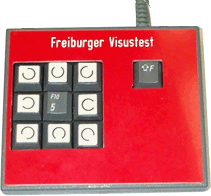
Another aspect: Some participants tend to press the keys for a prolonged time, triggering keyboard autorepeat, thus causing inadvertent response errors. Here it helps to switch off keyboard repeat through the appropriate facilities of your operating system.

I am lazy and prefer to start actions without mousing, thus I added a number of shortcuts.

Avoiding more mousing: Use the tab key (⇥) to move between textfields in Settings (shift-tab for backwards). The blue 🆗 button is activated by the ␍<return> key (⮐).

The manual of the previous, “classic” FrACT3.10.5, is here: PDF. The current version of FrACT₁₀ is here.

• Bach M (1996) The “Freiburg Visual Acuity Test” – Automatic measurement of visual acuity. Optometry and Vision Science 73:49–53
• Bach M (1997) Anti-aliasing and dithering in the “Freiburg Visual Acuity Test’. Spatial Vision 11:85–89
• Bach M (2007) The Freiburg Visual Acuity Test – Variability unchanged by post-hoc re-analysis. Graefe’s Arch Clin Exp Ophthalmol 245:965–971
• Bach M, Schäfer K (2016) Visual acuity testing: feedback affects neither outcome nor reproducibility, but leaves participants happier. PLOS ONE 11(1):e0147803
• Committee on Vision (1980) Recommended standard procedures for the clinical measurement and specification of visual acuity. Adv Ophthalmol 41:103–148
• International Organization for Standardization. ISO 8596:2019 Ophthalmic optics—Visual acuity testing—Standard optotype and its presentation
• Hamm LM, Yeoman JP, Anstice N, Dakin SC (2018) The Auckland Optotypes: An open-access pictogram set for measuring recognition acuity. JOV 18:13 DOI
• Sloan LL (1959) New test charts for the measurement of visual acuity at far and near distances. Am J Ophthalmol 48:807–813

• 2024-03-31 add Dithering and some contrast details
• 2024-02-18 add several small recent additions, and section on optimal optotype size for contrast testing
• 2024-01-22 revised license info
• 2024-01-16 explain Contrast Sensitivity ↔ Threshold Contrast
• 2023-08-03 extended Shortcuts
• 2023-07-06 mention of zoom levels in the operating system
• 2023-05-07 added Gratings
• 2023-02-08 added Autorun
• 2022-10-31 added info on in “inch” field
• 2022-10-27 renamed credit card to plastic card
• 2022-07-18 revised the VDU limitations section, also giving more manufacturer suggestions.
• 2022-05-22 added “Starting LogMAR”
• 2022-05-02 added “Margin for biggest optotype”
• 2022-03-02 added credit card calibration method
• 2022-01-07 added example R code to parse the “full history” export
• 2022-01-05 added “halfCI95”, “decimal separator” rather than “decimal mark character”
• 2021-12-23 added “Line of optotypes”
• 2021-12-07 added field “→min possible LogMAR”
• 2021-09-16 added window background color setting; mentioned Oblique only setting
• 2021-08-01 documented new eccentricity option; some stylistic editing
• 2021-07-04 changed the “empty fields” entry, because problem solved
• 2021-05-26 stylistic improvements, added shortcuts and CI95
• 2021-02-21 added gamma and many details
• 2020-11-10 added new settings, corrected types, rewording
• 2020-09-29 added details on contrast assessment
• 2020-07-03 mirrored one GUI word change, added export Vs2 with decimalMark, automated version date
• 2020-06-24 improved style, improved result export description, added keyboard pictures & shortcuts
• 2020-06-17 added volume slider, removed “draft” qualifier
• 2020-06-12 filled in missing details, added crowding
• 2020-06-10 started from the previous (FrACT3.10…) version.