
Well, the title may be a bit too grandiose, but my little investigation may surprise you too.
When I read a paper stating “We were able to show…” I cringe (and I delete it from any papers I co-author). To simplify, there are two ways to do science. Approach A is to “… perceive whatever holds / The world together in its inmost folds”, approach B: “look how much work/ingenuity I have invested / impact factor harvested / publications put out / recognition earned” (yes I said it’s simplified ;-). So for me approach A is typified by “We found…”, while approach B is revealed by “We were able to show…”. Now I know myself – I can go overboard with my opinions. So in my last sleepless night it occurred to me to look whether my feeling that everyone these days is “able to show / demonstrate…” is just my obsession or based on actual fact. So I went to Google Scholar, where it is easy to narrow searches to time ranges, and compared the number of occurrences of “we found” versus “we were able to show”.
Based on a quick web query I learned the term “web scraper” and built a simple one to extract the number of results. [This is “iffed out” in the code below, since it banned me after a few tries – see comments on “scraping” Google Scholar; ideas?]
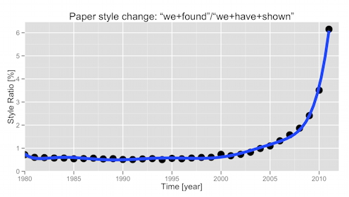
Amazingly: the ratio of “we could show” over “we found” changed from 0.5–0.7% in 1980–2000 to 6% in 2011, a 8th(!) order polynom being necessary to model the steep rise by a factor of 10 in the last ≈5 years!
There’s lots to be argued – is the wording I chose adequate, is it occasionally ok to say “we could show…” (yes), why I started 1980, and and… This post is already too long. Finally, here’s the code, and I would love to learn how to improve (e.g. get rid of the for loop) and how to avoid a Google ban (which shows up as “this page has moved”).
Code Begin
#
looking for a style change in scientific papers over time
#
© 2012-08-05 Michael Bach
«a href=”https://michaelbach.de”>https://michaelbach.de</a>> bach@uni-freiburg.de
#
a simple scholar scraper
googleScholarHits <- function(searchString, yearStart, yearEnd) {
require(RCurl)

url = paste0("<a href="http://scholar.google.com/scholar?as_ylo=">http://scholar.google.com/scholar?as_ylo=</a>",

	as.character(yearStart), "&as_yhi=",  as.character(yearEnd),

	"&q=%22", searchString, "%22&hl=en&num=1&as_sdt=0")

print(url)

webpage = as.character(getURL(url))

print(substr(webpage, 1, 500))

require(stringr)

start = str_locate(webpage, fixed(">About "))[2]

end = str_locate(webpage, fixed(" results ("))[1]

number = substr(webpage, start, end)

return(as.numeric(sub(pattern=",", replacement="", x=number)))
}
style1string=”we+found”; style2string=”we+have+shown”
googleScholarHits(style1string, 2009, 2009) # a manual test
years = seq(from=1980, to=2011, by=1)
if (FALSE) {
nStyle1 = array();  nStyle2 = array();  i = 1

for (year in years) {

	nStyle1[i] = googleScholarHits(style1string, year, year)

	nStyle2[i] = googleScholarHits(style2string, year, year)

	i = i+1;

}

d = data.frame(years, nStyle1, nStyle2)
} else {
since the scraper caused Google to “ban” me, here are the literal findings
dRaw = "year	nStyle1	nStyle2

1980	39200	282

1981	44400	268

1982	49400	292

1983	56000	321

1984	61600	352

1985	66300	359

1986	72300	397

1987	79000	448

1988	87300	466

1989	96500	528

1990	109000	558

1991	115000	583

1992	123000	657

1993	135000	739

1994	146000	737

1995	158000	880

1996	168000	907

1997	176000	1010

1998	185000	1110

1999	196000	1190

2000	218000	1600

2001	214000	1440

2002	218000	1600

2003	225000	1860

2004	229000	2260

2005	215000	2360

2006	204000	2690

2007	187000	2950

2008	170000	3170

2009	146000	3520

2010	102000	3580

2011	64200	3950"

d = read.table(textConnection(dRaw), header=TRUE)
}
d$nStylesRatio = d$nStyle2 / d$nStyle1
library(ggplot2); library(scales)
ggplot(data=d, aes(x=years, y=nStylesRatio)) +
geom_point(size=5) +
stat_smooth(method = “lm”, formula=y ~ poly(x, 8), size=2) +
scale_y_continuous(labels=percent) +
coord_cartesian(xlim=c(1980, max(years)+1), ylim=c(0, 1.05*max(d$nStylesRatio, na.rm=T))) +
labs(x=”Time [year]”, y = “Style Ratio [%]”) +
opts(title = paste0(“Paper style change: “”, style1string, “”/“”, style2string,”””))
#